 srcmini
本文概述
- 安装和演示数据集
- 1.默认情况下急切执行
- 2. tf.function和AutoGraph
- 3.不再需要tf.variable_scope
- 4.自定义图层非常简单
- 5.模型训练的灵活性
- 6. TensorFlow数据集
- 7.自动混合精度策略
- 8.分布式训练
- 9. Jupyter Notebook中的TensorBoard
- 10. TensorFlow for Swift
- 下一步是什么?
TensorFlow 2.0 alpha已发布。该框架确实对深度学习社区产生了重大影响。从业者, 研究人员, 开发人员都喜欢该框架, 并且从未像现在这样对其进行过调整。这很容易是我们今天看到的所有超酷深度学习启用应用程序迅速启动的主要原因之一。话虽如此, TensorFlow 1.x也有其缺点(就像许多其他框架一样)。正如Martin Wicke(TensorFlow团队的软件工程师)在TF Dev Summit ’19上所说的那样-
从1.0开始, 我们学到了很多东西。
从广泛的用户群, GitHub问题中吸取的所有教训之后, TensorFlow团队发布了TensorFlow 2.0 alpha, 该版本进行了许多重要的改进, 以改善性能, 用户体验等。它使你能够快速制作原型, 并包括许多现代深度学习实践。在本文中, 你将通过精确的实现来研究其中的一些更改。
请注意, 根据作者的说法, 此处讨论的更新是最重要的更新。你需要具备一些TensorFlow和Keras的经验, 才能继续阅读本文。以下是一些资源, 在TensorFlow和Keras上进行复习时, 你可能会发现它们很方便-
- TensorFlow初学者教程
- Keras教程:Python深度学习
安装和演示数据集
更新到TensorFlow 2.0是从Jupyter Notebook运行以下代码行:
!pip install tensorflow == 2.0.0-alpha0
GPU变体也可以以相同的方式安装(之前需要CUDA):
!pip install tensorflow-gpu == 2.0.0-alpha0
你可以在此处找到有关安装过程的更多信息。
你将要研究的一些更新包括代码实现。在这种情况下, 你将需要一个数据集。对于本文, 你将使用UCI存档中的Adult数据集。
import pandas as pd

columns = ["Age", "WorkClass", "fnlwgt", "Education", "EducationNum", "MaritalStatus", "Occupation", "Relationship", "Race", "Gender", "CapitalGain", "CapitalLoss", "HoursPerWeek", "NativeCountry", "Income"]

data = pd.read_csv('https://archive.ics.uci.edu/ml/machine-learning-databases/adult/adult.data', header=None, names=columns)

data.head()
| 年龄 | 工作班级 | fnlwgt | 教育 | 教育数字 | 婚姻状况 | 占用 | 关系 | 种族 | 性别 | 资本收益 | 资本损失 | 每周几小时 | 祖国 | 收入 | |
|---|---|---|---|---|---|---|---|---|---|---|---|---|---|---|---|
| 0 | 39 | 国家政府 | 77516 | 学士学位 | 13 | 从未结婚 | 副书记 | 不在家庭中 | 白色 | 男 | 2174 | 0 | 40 | 美国 | <= 50K |
| 1 | 50 | 自我-没有收入 | 83311 | 学士学位 | 13 | 已婚公民配偶 | 行政管理 | 丈夫 | 白色 | 男 | 0 | 0 | 13 | 美国 | <= 50K |
| 2 | 38 | private | 215646 | HS-城市 | 9 | 离婚了 | 搬运清洁工 | 不在家庭中 | 白色 | 男 | 0 | 0 | 40 | 美国 | <= 50K |
| 3 | 53 | private | 234721 | 11日 | 7 | 已婚公民配偶 | 搬运清洁工 | 丈夫 | 黑色 | 男 | 0 | 0 | 40 | 美国 | <= 50K |
| 4 | 28 | private | 338409 | 学士学位 | 13 | 已婚公民配偶 | 专业 | 妻子 | 黑色 | 女 | 0 | 0 | 40 | 古巴 | <= 50K |
该数据集表示一个二进制分类任务, 该任务将预测一个人每年的收入是否超过5万美元, 或者没有给出一组个人详细信息。
让我们进行一些基本的数据预处理, 然后以80:20的比例设置数据拆分:
from sklearn.preprocessing import LabelEncoder
from sklearn.model_selection import train_test_split
import numpy as np

# Label Encode
le = LabelEncoder()
data = data.apply(le.fit_transform)

# Segregate data features & convert into NumPy arrays
X = data.iloc[:, 0:-1].values
y = data['Income'].values

# Split
X_train, X_test, y_train, y_test = train_test_split(X, y, test_size=0.2, random_state=7)
到现在为止, 你应该已经安装了TensorFlow 2.0并在工作区中加载了数据集。现在, 你可以继续进行更新。
1.默认情况下急切执行
在TensorFlow 2.0中, 你不再需要创建会话并在其中运行计算图。在2.0版中, 默认情况下, 急切执行是启用的, 因此你可以构建模型并立即运行它们。你可以选择禁用急切执行, 如下所示:
tf.compat.v1.disable_eager_execution()(提供的张量流使用tf别名导入。)
这是一个基于代码的比较, 表明了这种差异-
2. tf.function和AutoGraph
尽管急切执行使你能够进行命令式编程, 但在分布式训练, 全面优化, 生产环境中, TensorFlow 1.x样式图执行具有优于急切执行的优势。在TensorFlow 2.0中, 你可以保留基于图的执行方式, 但使用方式更加灵活。它是通过tf.function和AutoGraph实现的。
tf.function允许你通过其AutoGraph功能使用Python样式的语法定义TensorFlow图。 AutoGraph支持广泛的Python兼容性, 包括if语句, for循环, while循环, 迭代器等。但是, 存在一些限制。在这里, 你可以找到当前可用的支持的完整列表。下面的示例向你展示了仅用装饰器定义TensorFlow图是多么容易。
import tensorflow as tf

# Define the forward pass
@tf.function
def single_layer(x, y):
    return tf.nn.relu(tf.matmul(x, y))

# Generate random data drawn from a uniform distribution
x = tf.random.uniform((2, 3))
y = tf.random.uniform((3, 5))

single_layer(x, y)
<tf.Tensor: id=73, shape=(2, 5), dtype=float32, numpy=
array([[0.5779363 , 0.11255255, 0.26296678, 0.12809312, 0.23484911], [0.5932371 , 0.1793559 , 0.2845083 , 0.23249313, 0.21367362]], dtype=float32)>
请注意, 你不必创建任何会话或占位符即可运行功能single_layer()。这是tf.function的漂亮功能之一。在后台, 它会进行所有必要的优化, 以使你的代码运行更快。
3.不再需要tf.variable_scope
在TensorFlow 1.x中, 为了能够将tf.layers用作变量并重用它们, 你必须使用tf.variable块。但这在TensorFlow 2.0中不再需要。由于TensorFlow 2.0中存在以keras为中心的高级API, 因此可以轻松地将使用tf.layers创建的所有图层放入tf.keras.Sequential定义中。这使代码更易于阅读, 并且你也可以跟踪变量和损失。
这是一个例子:
# Define the model
model = tf.keras.Sequential([
    tf.keras.layers.Dropout(rate=0.2, input_shape=X_train.shape[1:]), tf.keras.layers.Dense(units=64, activation='relu'), tf.keras.layers.Dropout(rate=0.2), tf.keras.layers.Dense(units=64, activation='relu'), tf.keras.layers.Dropout(rate=0.2), tf.keras.layers.Dense(units=1, activation='sigmoid')
])

# Get the output probabilities
out_probs = model(X_train.astype(np.float32), training=True)
print(out_probs)
tf.Tensor(
[[1.        ]
 [0.12573627]
 [1.        ]
 ...
 [1.        ]
 [1.        ]
 [1.        ]], shape=(26048, 1), dtype=float32)
在上面的示例中, 你通过模型传递了训练数据, 只是为了获得原始输出概率。注意, 这只是一个前向通过。你当然可以继续进行模型训练-
model.compile(loss='binary_crossentropy', optimizer='adam')

model.fit(X_train, y_train, validation_data=(X_test, y_test), epochs=5, batch_size=64)
Train on 26048 samples, validate on 6513 samples
Epoch 1/5
26048/26048 [==============================] - 2s 62us/sample - loss: 79.5270 - val_loss: 0.7142
Epoch 2/5
26048/26048 [==============================] - 1s 48us/sample - loss: 2.0096 - val_loss: 0.5894
Epoch 3/5
26048/26048 [==============================] - 1s 47us/sample - loss: 0.8750 - val_loss: 0.5761
Epoch 4/5
26048/26048 [==============================] - 1s 49us/sample - loss: 0.6650 - val_loss: 0.5629
Epoch 5/5
26048/26048 [==============================] - 1s 47us/sample - loss: 0.6885 - val_loss: 0.5539


<tensorflow.python.keras.callbacks.History at 0x7fc2b1944780>
你可以按以下方式逐层获取模型的可训练参数的列表:
# Model's trainable parameters in a layer by layer fashion
model.trainable_variables
[<tf.Variable 'dense_12/kernel:0' shape=(14, 64) dtype=float32, numpy=
 array([[-1.48688853e-02, 2.74527162e-01, 2.58149177e-01, -2.35980123e-01, 7.92130232e-02, -1.19770452e-01, 1.83823228e-01, 2.26748139e-01, -1.31252930e-01, -1.67176753e-01, 1.43430918e-01, 2.32805759e-01, 2.47395486e-01, 8.89694989e-02, 1.75705254e-02, -2.01672405e-01, 2.01087326e-01, -1.67460442e-01, -1.03051037e-01, -2.56078333e-01, -6.07236922e-02, 4.76933420e-02, -4.65645194e-02, 2.20712095e-01, 1.98741913e-01, 9.32294428e-02, 1.51318759e-01, -3.96257639e-03, -1.51869521e-01, 8.89182389e-02, -4.22340333e-02, 1.55168772e-03, -7.01716542e-03, -8.23616534e-02, -1.85766399e-01, -1.97881564e-01, 1.94241285e-01, 2.11566478e-01, -1.68947518e-01, -2.34904587e-01, -8.28040987e-02, -1.37671828e-02, 3.46715450e-02, 9.42899585e-02, 9.07505751e-02, 2.64314085e-01, 4.13734019e-02, -1.75569654e-02, 2.49794573e-01, 2.40060896e-01, 1.24608070e-01, -2.27075279e-01, -1.13472998e-01, -1.09154880e-01, -2.51923293e-01, 2.43190974e-01, 2.63507813e-01, 1.83881164e-01, 5.65617085e-02, -2.68286765e-01, 1.78039759e-01, 6.91905916e-02, -2.60141104e-01, -2.56884694e-02], [-1.60553172e-01, 1.84462130e-01, -1.64327353e-01, -2.02879310e-03, -1.35839581e-02, -2.11382195e-01, -1.51656792e-01, -1.50204003e-02, 1.61570847e-01, -1.29508615e-01, -1.70697004e-01, -2.11556107e-01, 2.15181440e-01, 2.67737001e-01, -1.19572535e-01, 1.15734965e-01, -5.27024269e-02, 4.56553698e-02, -1.80567816e-01, -1.51056111e-01, -2.31304854e-01, -1.31544277e-01, 1.42878979e-01, -8.88223648e-02, -2.77194977e-01, 1.98713481e-01, 1.64229482e-01, -8.50015134e-02, 1.04941219e-01, 2.73275048e-01, 2.01503932e-02, 2.22145498e-01, 1.61160469e-01, 5.18816710e-02, -1.18925110e-01, 2.20809698e-01, 9.16796625e-02, -1.24019340e-01, -1.42927185e-01, -1.58376783e-01, 8.95256698e-02, -1.36581853e-01, -9.74076241e-02, -2.06318110e-01, 4.34296429e-02, 1.48526222e-01, -2.64008492e-01, 2.33468860e-01, -1.74503058e-01, -2.60894388e-01, 1.12190038e-01, -1.72933638e-01, 1.87754840e-01, 5.69777489e-02, 9.31494832e-02, 9.37287509e-02, -2.24829912e-01, -5.65375686e-02, -2.31988132e-01, -5.92674166e-02, -2.54451334e-01, -1.28820181e-01, 1.57452404e-01, 2.53181010e-01], [-8.94532055e-02, -7.04574287e-02, -2.74045289e-01, -2.29278371e-01, -1.12556815e-02, -4.37867343e-02, 6.96483850e-02, -2.20679641e-02, -8.04719925e-02, -4.27710414e-02, -6.98548555e-03, 5.35116494e-02, -1.54523849e-02, -1.36115998e-01, 1.38038993e-01, -1.85180068e-01, 2.15847164e-01, 2.55365819e-01, 1.37135267e-01, 1.90906912e-01, -2.23682523e-02, 1.52650058e-01, 2.04477787e-01, -4.36266363e-02, 1.78499818e-01, 1.90241158e-01, -2.02745885e-01, 1.43350720e-01, -1.13368660e-01, -2.01326758e-01, -1.61648542e-01, 2.25443751e-01, -2.68535197e-01, 2.37828940e-01, 2.71143168e-01, 1.59860253e-02, 1.41094506e-01, -1.76632628e-01, 1.88476801e-01, 2.02816904e-01, -1.03268191e-01, -2.36591846e-01, 1.79396987e-01, 1.70014054e-01, -2.30597705e-01, 2.61288881e-03, -4.42424417e-03, -3.84955704e-02, 2.72334903e-01, -4.91250306e-02, 1.07610583e-01, -2.72850186e-01, -2.71188200e-01, -1.15645885e-01, 2.53611356e-01, -1.48682937e-01, -4.46224958e-02, -6.12093955e-02, -2.67423481e-01, -1.97976261e-01, 4.02505398e-02, 8.28173161e-02, 1.94115847e-01, 6.79514706e-02], [ 1.02568567e-02, -2.73051471e-01, 1.93972498e-01, 1.67789280e-01, -7.65820295e-02, 1.69053733e-01, -1.67652726e-01, -1.12306148e-01, 1.29045337e-01, 5.20431995e-03, 1.22617424e-01, 2.59980887e-01, 2.37120360e-01, 2.59193987e-01, 1.71425581e-01, 2.73495167e-01, -3.11368108e-02, 2.11496860e-01, -2.26072937e-01, -9.43622887e-02, 2.56022662e-01, 1.86894894e-01, -2.35674426e-01, -9.95516777e-03, 1.84704363e-01, 2.27636904e-01, -1.74311996e-02, -1.57380402e-02, -1.43433169e-01, -1.87973380e-02, 1.76340997e-01, -1.85148180e-01, 1.91334367e-01, 1.00137413e-01, -2.62901902e-01, -8.22693110e-03, -1.17425114e-01, -2.61702567e-01, -2.40183711e-01, -7.42957443e-02, -2.43198499e-01, 1.00527972e-01, -1.11117616e-01, -9.74197388e-02, -1.09167382e-01, -7.14137256e-02, 2.48018056e-01, -3.86851579e-02, 4.26724553e-02, -2.99333185e-02, 2.41537303e-01, -2.68284887e-01, 8.95127654e-03, -3.74048352e-02, 4.77899015e-02, 2.41122097e-01, 1.11537516e-01, -3.37415487e-02, -1.43319309e-01, -1.34244651e-01, 1.61695689e-01, -1.83817685e-01, 5.05107641e-02, 2.74721473e-01], [ 3.05238366e-02, 4.31960225e-02, 1.15660310e-01, 2.01156676e-01, 8.93190503e-03, -1.82507738e-01, -1.66644901e-01, 2.53293186e-01, 9.39259827e-02, 2.66437620e-01, 1.03438407e-01, 6.01558089e-02, -5.76229393e-02, 1.00222319e-01, -8.71886164e-02, 2.47991115e-01, 2.03391343e-01, -5.64218462e-02, -1.81319863e-01, -1.78091347e-01, 1.94970667e-02, 2.73696750e-01, 2.22271591e-01, -1.62375182e-01, -1.20849550e-01, -5.32025993e-02, -7.60249197e-02, -3.30891609e-02, -1.34273469e-01, -7.55624324e-02, 1.07143939e-01, 2.12463081e-01, 7.97367096e-03, -6.87274337e-03, -8.43367577e-02, 2.55893081e-01, 1.24732047e-01, 3.09056938e-02, 8.86841714e-02, -2.23312736e-01, 1.97805136e-01, 2.18041629e-01, 3.45717669e-02, -4.20909375e-02, 5.96292019e-02, 1.79306090e-01, 2.72990197e-01, 3.02815437e-02, 2.37860054e-01, 2.76284903e-01, 3.77161503e-02, 2.26478606e-01, 8.85216296e-02, -1.82998061e-01, -1.41343147e-01, -3.46849561e-02, -2.34851494e-01, 1.46038651e-01, -1.52093291e-01, -8.06826651e-02, 8.09380412e-03, 2.53538191e-02, -1.27880573e-02, 1.55383885e-01], [-1.07118145e-01, 2.71667391e-01, -1.35462150e-01, 8.78523886e-02, 8.47310722e-02, -3.18741649e-02, -1.72285080e-01, 9.50790346e-02, -7.42185712e-02, -1.69902325e-01, -8.20439905e-02, -3.02564055e-02, 1.61808312e-01, 6.13009930e-03, 4.78896201e-02, -1.39527738e-01, -1.96388185e-01, -9.79056209e-02, 8.11750889e-02, -8.75651240e-02, -3.17215472e-02, 2.24185854e-01, 1.03506386e-01, 2.46435404e-03, -1.83918521e-01, -1.77772760e-01, -1.59666687e-01, -5.00660688e-02, -1.95413038e-01, 2.49774963e-01, 2.11800635e-01, 7.34189749e-02, -1.63613647e-01, 1.28584713e-01, -2.04943165e-01, 4.48526740e-02, -9.40444320e-02, -2.36514211e-01, 4.40850854e-02, -7.21262991e-02, 5.26860356e-03, 2.54257828e-01, -1.71898901e-02, -1.66287631e-01, -4.29128110e-02, 3.84885073e-02, 1.63391858e-01, -1.09616295e-01, 2.26927966e-01, -2.67344981e-01, 1.98232234e-01, 1.29737794e-01, 2.69295484e-01, -2.23180622e-01, -1.87438726e-03, -5.20526767e-02, 9.74531174e-02, -1.05390891e-01, 1.23165011e-01, 2.33101934e-01, -2.56039590e-01, 2.46387571e-01, 1.33860320e-01, 1.71753883e-01], [ 2.46957332e-01, -4.92525846e-02, -2.22080618e-01, 4.05346751e-02, -5.00992537e-02, -2.60361612e-01, 1.50414556e-01, 2.01799482e-01, -2.87890434e-03, 9.51286852e-02, -5.86918592e-02, 2.12740213e-01, -1.76745623e-01, -2.74649799e-01, 2.05127060e-01, -4.51588929e-02, -1.18441284e-02, 1.17566496e-01, 2.14967847e-01, 2.30442315e-01, -2.03341544e-02, 7.21938014e-02, 1.91002727e-01, -2.73522615e-01, -1.07315734e-01, 1.57117695e-01, -7.27429241e-02, 1.98784769e-01, 1.34299874e-01, -2.60534406e-01, 8.44456553e-02, 5.92016876e-02, -8.88088793e-02, 9.40183103e-02, 8.87127221e-02, -9.60084200e-02, 2.42618769e-01, 9.65010524e-02, 6.18630648e-03, 1.61135674e-01, -3.82966697e-02, 1.02110088e-01, -1.88043356e-01, 6.97199404e-02, 2.39620298e-01, 5.69199026e-02, -1.25965476e-01, -8.32125545e-02, -8.48805904e-03, 1.70814633e-01, 2.38609940e-01, 9.24529135e-02, 9.29380953e-02, -1.60003811e-01, -2.04197079e-01, 2.51140565e-01, 2.41884738e-01, -2.46104851e-01, 6.61611557e-03, -2.67855734e-01, -7.67029077e-02, -2.74775296e-01, 2.36378461e-01, -2.72717297e-01], [ 1.63002580e-01, -1.04987592e-01, -1.11121044e-01, -2.73849100e-01, 1.99946165e-02, 2.11521506e-01, 2.06256032e-01, 2.54784852e-01, 2.57405788e-01, 1.75982475e-01, -1.57612175e-01, -1.88202858e-02, -1.82799488e-01, -6.26320094e-02, -9.18765068e-02, -1.66230381e-01, 2.42929131e-01, -3.45604420e-02, 3.02044451e-02, -1.67087615e-02, -9.18568671e-02, -1.18204534e-01, 2.26822466e-01, -8.45120549e-02, 1.58829272e-01, -2.22656310e-01, -1.80833176e-01, -1.51249528e-01, 2.30215102e-01, -2.01435268e-01, 2.50793129e-01, 1.61696225e-01, 1.12378091e-01, -8.44676197e-02, -1.86490998e-01, 2.16112882e-01, -1.67694584e-01, 8.36035609e-02, 1.36310160e-02, -2.36266181e-01, 2.16432512e-02, 2.17068702e-01, 1.48556292e-01, -6.13741130e-02, 1.84532225e-01, -1.20505244e-01, 5.50346076e-02, 1.04375720e-01, 1.96388662e-01, 2.04656780e-01, 8.99768472e-02, 1.04485691e-01, 1.16647959e-01, -9.09715742e-02, 2.40128249e-01, 7.08191991e-02, -1.35386303e-01, 1.52992904e-02, 2.04906076e-01, 2.08586067e-01, 2.65424818e-01, 1.74420804e-01, 1.45571589e-01, -1.06450215e-01], [-1.22071415e-01, 6.90596700e-02, -9.81627107e-02, -1.82385862e-01, 3.71887982e-02, 1.33560777e-01, 6.62094355e-03, -2.25594267e-01, -8.94398540e-02, -2.11033255e-01, 2.53058523e-01, 5.08429706e-02, -1.27695456e-01, -7.27435797e-02, -1.51305407e-01, 3.16268504e-02, 2.58970231e-01, 8.51702690e-02, 2.73242801e-01, -1.25677899e-01, -2.71640301e-01, -1.60824418e-01, -2.76342273e-01, 2.24858135e-01, -8.03019106e-02, -4.79616970e-02, 4.94971275e-02, 2.46035010e-01, -1.74869299e-02, 1.85437828e-01, -2.01017499e-01, -2.23311543e-01, 2.70765752e-01, -2.11389661e-01, -2.26453170e-01, 2.06002831e-01, 2.16605961e-01, 1.56077802e-01, -2.76331574e-01, -7.14364648e-03, -1.25960454e-01, 1.02812976e-01, 5.37744164e-03, -9.14498568e-02, -2.16731012e-01, -4.22561914e-02, -1.18804276e-02, -4.11395282e-02, -2.58837283e-01, -9.24162269e-02, 2.24286765e-01, 1.97664350e-01, -2.04566836e-01, 1.49493903e-01, 1.82809919e-01, 2.18066871e-01, 2.27073222e-01, 1.76770508e-01, 1.28788888e-01, 7.43162632e-03, -2.44799465e-01, 2.06821591e-01, -9.25005376e-02, 1.84141576e-01], [ 1.05317682e-01, 1.83150172e-02, -6.71321154e-02, 1.00300103e-01, -2.54237145e-01, -3.71084660e-02, -1.02833554e-01, -5.97543716e-02, -2.18547538e-01, -8.90600234e-02, -2.40394264e-01, -2.57878542e-01, -1.38011947e-01, 2.36597955e-02, -2.27259427e-01, -1.65269971e-02, 2.32348710e-01, -1.00096032e-01, -2.13123351e-01, -1.40784979e-02, -2.66731352e-01, -2.15898558e-01, -5.78602701e-02, 1.08396888e-01, -2.02795267e-01, -1.52687684e-01, 2.78952122e-02, 4.09219265e-02, -5.15770912e-02, -1.81588203e-01, 2.73707718e-01, 1.09840721e-01, -1.40243679e-01, -2.13766873e-01, -1.94679320e-01, -9.15652514e-03, -1.61587566e-01, 2.27655083e-01, -1.11349046e-01, -1.05967700e-01, 8.99270475e-02, 2.07172066e-01, 5.06473184e-02, 2.01718628e-01, -1.03773981e-01, 2.73704678e-01, 4.07311916e-02, 9.41670239e-02, -7.51210451e-02, 2.25694746e-01, 4.44093049e-02, 2.77287036e-01, 2.25879252e-02, -6.58842623e-02, -2.06691712e-01, -1.68207854e-01, 1.10538006e-02, -1.19143382e-01, 1.65247411e-01, -1.02170840e-01, 7.17070699e-02, -7.43492991e-02, -7.37106651e-02, -1.29226327e-01], [ 2.08517313e-02, 8.65581036e-02, -2.01248676e-01, -1.06920242e-01, 2.04556465e-01, -5.12601584e-02, 1.17174774e-01, -1.21960059e-01, -1.31039545e-01, 1.45936877e-01, 9.38895345e-03, -1.14137828e-02, 1.54711992e-01, 2.67244726e-01, -7.15402961e-02, -2.23028928e-01, -2.71299481e-01, -1.36449203e-01, -1.25627816e-02, 3.13916504e-02, 1.73118323e-01, -2.17780888e-01, -1.95076853e-01, 1.28784478e-02, 1.73919499e-01, -2.42948875e-01, -2.14346394e-01, 5.35857081e-02, 2.67256826e-01, -1.71346068e-02, -2.76432812e-01, -1.73468918e-01, 1.22662723e-01, -9.96078849e-02, -1.15638345e-01, -2.65158296e-01, 2.12729961e-01, -2.70184338e-01, 1.08982086e-01, -1.14385784e-02, 2.67733067e-01, 2.64605552e-01, 7.57011771e-02, -8.78878832e-02, -9.69131440e-02, -6.81236386e-03, 6.40029907e-02, -1.91579491e-01, 1.71635926e-01, -2.19610840e-01, -1.01383820e-01, 1.74940199e-01, -1.23514935e-01, -4.02086824e-02, 2.65191942e-01, -2.47828737e-01, -5.83019853e-03, -1.24326095e-01, -2.10787788e-01, -2.57244408e-02, -9.65181738e-02, -1.34586707e-01, -2.63660282e-01, -2.33780265e-01], [-2.09537894e-01, 1.81803823e-01, -2.23274127e-01, 2.68277794e-01, -2.12194473e-01, 2.69619197e-01, -1.91460058e-01, 1.50443584e-01, -6.01146221e-02, 1.15322739e-01, 5.74926138e-02, -2.09335685e-01, 2.66064018e-01, -2.50099152e-01, 2.27989703e-01, 1.48722529e-03, -2.75823861e-01, -2.74460733e-01, -2.54678339e-01, 2.07069367e-01, 2.42757052e-01, -8.09566826e-02, -2.22230926e-01, 3.88453007e-02, -7.51499534e-02, -1.13763615e-01, 1.86943352e-01, 1.81314886e-01, -1.03227988e-01, 1.27721041e-01, 1.00327253e-01, -1.25737816e-01, -9.31653380e-03, -1.79606676e-02, -1.99202478e-01, 1.40470475e-01, -1.78151071e-01, 3.56182456e-02, 2.09965855e-01, 9.80757773e-02, 9.55764055e-02, 2.42440253e-01, 2.26146430e-01, -8.72465968e-03, -2.06995502e-01, 1.26261711e-01, 1.92399114e-01, 2.21498907e-02, 2.40556687e-01, -1.17468238e-01, -8.96153450e-02, 3.64099145e-02, 5.64157963e-05, -9.97322649e-02, 1.81693852e-01, -1.95398301e-01, 2.67696530e-01, 2.18172163e-01, 1.50565267e-01, -2.76668876e-01, -2.90721059e-02, 6.15487993e-02, 5.47989309e-02, -2.45864540e-01], [ 1.13498271e-01, -1.24701887e-01, -1.19635433e-01, 6.81682229e-02, 1.42366707e-01, -5.18653989e-02, 1.70933545e-01, 4.18927073e-02, -8.23812187e-02, -1.72122866e-01, 3.46628726e-02, 2.39999801e-01, -4.86224890e-04, 8.29051435e-02, -6.71084374e-02, -1.72895417e-01, -2.63225108e-01, -1.55994743e-01, 8.19830298e-02, 2.49279350e-01, -1.41113624e-01, 1.25947356e-01, -9.30310488e-02, 2.40998656e-01, 2.44344383e-01, -1.36330962e-01, -1.14291891e-01, -2.29074568e-01, 1.76846683e-01, -7.63051659e-02, -6.28410280e-02, -1.43780455e-01, -7.99130350e-02, -2.32542127e-01, -3.03542614e-03, 7.96765089e-03, 2.05407441e-02, -3.18776071e-02, -1.66951925e-01, -2.53402591e-01, 1.85931325e-02, -2.08924711e-02, -2.02480197e-01, -1.78624660e-01, -9.39854980e-03, 2.22942740e-01, -7.72327036e-02, 8.92090797e-03, 5.94776869e-03, -1.45615578e-01, -1.00357220e-01, -6.98443055e-02, -1.69289708e-02, 1.10462517e-01, -2.50632793e-01, 1.05173588e-01, -1.03613839e-01, -1.78682446e-01, -4.74603325e-02, 2.64549822e-01, 2.41646737e-01, -9.74451900e-02, -1.91499934e-01, -2.03671366e-01], [ 3.43604088e-02, -4.77244258e-02, -2.74687082e-01, 1.44897908e-01, 1.87038392e-01, -2.73052067e-01, -1.34714529e-01, -1.96854770e-02, 1.78879768e-01, -4.30725813e-02, -1.44803524e-02, -4.08369452e-02, 1.24610901e-01, 1.33537620e-01, -5.67995459e-02, 1.66517943e-01, 1.21737421e-02, -2.28156358e-01, 2.42469996e-01, -8.04692805e-02, 2.54256994e-01, 1.89271569e-02, 1.06245875e-01, 2.76879996e-01, 1.47841871e-01, -9.83145386e-02, 1.41099930e-01, -9.15518403e-03, 2.22966105e-01, 1.95244431e-01, 2.46362776e-01, 1.43388927e-01, 2.12212205e-01, -2.39929557e-02, 2.23469466e-01, 2.43519396e-01, 2.35615760e-01, -7.24931657e-02, -9.37553197e-02, 2.35618442e-01, 1.09928012e-01, -2.83769220e-02, -1.05210841e-02, -2.18923137e-01, -1.58438280e-01, -1.87489986e-02, 1.51137710e-02, 1.77096963e-01, 7.83360600e-02, 2.20489174e-01, -3.45443189e-02, 6.89106286e-02, 2.31777161e-01, -1.25984594e-01, 1.43728256e-02, 2.55063027e-01, -2.42056713e-01, 8.74229670e-02, 2.20979035e-01, -2.00921297e-03, 1.69425875e-01, -8.34510028e-02, -1.03761226e-01, 8.88096690e-02]], dtype=float32)>, <tf.Variable 'dense_12/bias:0' shape=(64, ) dtype=float32, numpy=
 array([0., 0., 0., 0., 0., 0., 0., 0., 0., 0., 0., 0., 0., 0., 0., 0., 0., 0., 0., 0., 0., 0., 0., 0., 0., 0., 0., 0., 0., 0., 0., 0., 0., 0., 0., 0., 0., 0., 0., 0., 0., 0., 0., 0., 0., 0., 0., 0., 0., 0., 0., 0., 0., 0., 0., 0., 0., 0., 0., 0., 0., 0., 0., 0.], dtype=float32)>, <tf.Variable 'dense_13/kernel:0' shape=(64, 64) dtype=float32, numpy=
 array([[ 0.20200957, 0.03036232, 0.11040972, ..., -0.21020778, 0.17196609, -0.03736575], [-0.2064129 , 0.13786067, 0.09109865, ..., -0.15494904, 0.09000905, -0.18967415], [-0.0387924 , -0.02436857, 0.16121905, ..., -0.1803377 , -0.00170219, 0.15630807], ..., [ 0.19548352, 0.10514452, -0.03767221, ..., 0.03404056, 0.02135798, 0.00550348], [-0.16041529, -0.07542154, -0.1700579 , ..., 0.00083075, 0.11576484, 0.08763643], [-0.09544714, 0.08534966, -0.06500863, ..., 0.04508607, -0.17440501, 0.1134396 ]], dtype=float32)>, <tf.Variable 'dense_13/bias:0' shape=(64, ) dtype=float32, numpy=
 array([0., 0., 0., 0., 0., 0., 0., 0., 0., 0., 0., 0., 0., 0., 0., 0., 0., 0., 0., 0., 0., 0., 0., 0., 0., 0., 0., 0., 0., 0., 0., 0., 0., 0., 0., 0., 0., 0., 0., 0., 0., 0., 0., 0., 0., 0., 0., 0., 0., 0., 0., 0., 0., 0., 0., 0., 0., 0., 0., 0., 0., 0., 0., 0.], dtype=float32)>, <tf.Variable 'dense_14/kernel:0' shape=(64, 1) dtype=float32, numpy=
 array([[ 0.17874134], [ 0.06660989], [ 0.2120269 ], [ 0.1908356 ], [-0.05980097], [ 0.2545969 ], [ 0.16937432], [ 0.28103924], [-0.301428  ], [-0.1401844 ], [-0.02959338], [ 0.10712665], [ 0.09891567], [-0.28661886], [ 0.28736794], [ 0.03912222], [-0.03885537], [-0.25707358], [-0.24519518], [ 0.11147693], [ 0.02554649], [-0.20881867], [ 0.00373942], [ 0.02928248], [ 0.09055263], [ 0.15126869], [-0.11197442], [ 0.23908103], [ 0.07320437], [-0.05635457], [ 0.14777556], [-0.17251213], [-0.02642217], [ 0.25192064], [-0.15656634], [-0.0924283 ], [-0.20901027], [-0.17767514], [-0.15508023], [ 0.06313407], [ 0.2708218 ], [-0.14065444], [ 0.12714231], [-0.05807959], [ 0.17975545], [ 0.19628727], [-0.24905266], [-0.12731928], [-0.15389986], [-0.15024558], [-0.08432762], [-0.28963754], [-0.07519016], [-0.04082993], [ 0.13681188], [ 0.18757123], [ 0.09581241], [ 0.09615937], [ 0.22277021], [ 0.2865938 ], [ 0.00316831], [-0.27389333], [-0.09506477], [ 0.01873708]], dtype=float32)>, <tf.Variable 'dense_14/bias:0' shape=(1, ) dtype=float32, numpy=array([0.], dtype=float32)>]
4.自定义图层非常简单
在机器学习研究中, 甚至在工业应用中, 通常需要编写自定义层来满足特定用例。 TensorFlow 2.0使得编写自定义层并将其与现有层一起使用非常容易。你还可以按任何方式自定义模型的前向传递。
为了创建自定义图层, 最简单的选择是从tf.keras.layers扩展Layer类, 然后相应地对其进行定义。你将创建一个自定义层, 然后定义其正向计算。以下是执行help(tf.keras.layers.Layer)的输出。它告诉你要完成此操作需要指定哪些内容:
从上述摘要中获取建议, 你将-
- 用输出数量定义构造函数
- 在build()方法中, 你将为图层添加权重
- 最后, 在call()方法中, 通过将矩阵乘法和relu()链接在一起来定义前向传递
class MyDenseLayer(tf.keras.layers.Layer):
    # Define the constructor
    def __init__(self, num_outputs):
        super(MyDenseLayer, self).__init__()
        self.num_outputs = num_outputs
    # Define the build function to add the weights
    def build(self, input_shape):
        self.kernel = self.add_variable("kernel", shape=[input_shape[-1], self.num_outputs])
    # Define the forward pass
    def call(self, input):
        matmul = tf.matmul(input, self.kernel)
        return tf.nn.relu(matmul)

# Initialize the layer with 10 output units
layer = MyDenseLayer(10)
# Supply the input shape
layer(tf.random.uniform((10, 3)))
# Display the trainable parameters of the layer
print(layer.trainable_variables)
[<tf.Variable 'my_dense_layer_7/kernel:0' shape=(3, 10) dtype=float32, numpy=
array([[ 0.43613756, 0.21344548, 0.37803996, 0.65583944, 0.11884308, 0.13909656, 0.30802298, 0.5313586 , 0.04967308, 0.32889426], [ 0.1680265 , -0.59944266, -0.4014195 , 0.14887196, 0.07071263, 0.37862527, -0.5822403 , -0.5963166 , 0.3106798 , 0.05353856], [-0.44345278, -0.23122305, -0.62959856, -0.43062705, 0.13194847, -0.60124606, -0.62745696, 0.12254918, -0.09806103, -0.45324165]], dtype=float32)>]
你可以通过扩展tf.keras中的Model类来构成多层。你可以在此处找到有关组成模型的更多信息。
5.模型训练的灵活性
TensorFlow可以使用自动微分来计算损失函数相对于模型参数的梯度。 tf.GradientTape在上下文中创建一个磁带, TensorFlow使用该上下文来跟踪从该磁带中的每次计算记录的梯度。为了理解这一点, 让我们通过扩展tf.keras.Model类以更底层的方式定义模型。
from tensorflow.keras import Model

class CustomModel(Model):
    def __init__(self):
        super(CustomModel, self).__init__()
        self.do1 = tf.keras.layers.Dropout(rate=0.2, input_shape=(14, ))
        self.fc1 = tf.keras.layers.Dense(units=64, activation='relu')
        self.do2 = tf.keras.layers.Dropout(rate=0.2)
        self.fc2 = tf.keras.layers.Dense(units=64, activation='relu')
        self.do3 = tf.keras.layers.Dropout(rate=0.2)
        self.out = tf.keras.layers.Dense(units=1, activation='sigmoid')

    def call(self, x):
        x = self.do1(x)
        x = self.fc1(x)
        x = self.do2(x)
        x = self.fc2(x)
        x = self.do3(x)
        return self.out(x)

model = CustomModel()
请注意, 此模型的拓扑与你先前定义的拓扑完全相同。为了能够使用自动微分训练该模型, 你需要以不同的方式定义损失函数和优化器-
loss_func = tf.keras.losses.BinaryCrossentropy()
optimizer = tf.keras.optimizers.Adam()
现在, 你将定义度量标准, 这些度量标准将用于衡量转向其训练的网络的性能。性能是指模型的损失和准确性。
# Average the loss across the batch size within an epoch
train_loss = tf.keras.metrics.Mean(name='train_loss')
train_acc = tf.keras.metrics.BinaryAccuracy(name='train_acc')

valid_loss = tf.keras.metrics.Mean(name='test_loss')
valid_acc = tf.keras.metrics.BinaryAccuracy(name='valid_acc')
tf.data提供了定义输入数据管道的实用方法。当你处理大量数据时, 这特别有用。
现在, 你将定义数据生成器, 它将在模型训练期间生成大量数据。
X_train, X_test = X_train.astype(np.float32), X_test.astype(np.float32)
y_train, y_test = y_train.astype(np.int64), y_test.astype(np.int64)
y_train, y_test = y_train.reshape(-1, 1), y_test.reshape(-1, 1)

# Batches of 64
train_ds = tf.data.Dataset.from_tensor_slices((X_train, y_train)).batch(64)
test_ds = tf.data.Dataset.from_tensor_slices((X_test, y_test)).batch(64)
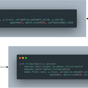
现在你可以使用tf.GradientTape训练模型了。首先, 你将定义一个方法, 该方法将使用你刚刚使用tf.data.DataSet定义的数据来训练模型。你还将使用tf.function装饰器包装模型训练步骤, 以利用其在计算中提供的加速。
模型训练与验证
# Train the model
@tf.function
def model_train(features, labels):
    # Define the GradientTape context
    with tf.GradientTape() as tape:
        # Get the probabilities
        predictions = model(features)
        # Calculate the loss
        loss = loss_func(labels, predictions)
    # Get the gradients
    gradients = tape.gradient(loss, model.trainable_variables)
    # Update the weights
    optimizer.apply_gradients(zip(gradients, model.trainable_variables))

    train_loss(loss)
    train_acc(labels, predictions)
# Validating the model
@tf.function
def model_validate(features, labels):
    predictions = model(features)
    t_loss = loss_func(labels, predictions)

    valid_loss(t_loss)
    valid_acc(labels, predictions)
使用以上两种方法来训练和验证5个时期的模型。
for epoch in range(5):
    for features, labels in train_ds:
        model_train(features, labels)

    for test_features, test_labels in test_ds:
        model_validate(test_features, test_labels)

    template = 'Epoch {}, train_loss: {}, train_acc: {}, train_loss: {}, test_acc: {}'
    print (template.format(epoch+1, train_loss.result(), train_acc.result()*100, valid_loss.result(), valid_acc.result()*100))
Epoch 1, train_loss: 9.8155517578125, train_acc: 66.32754516601562, train_loss: 2.8762073516845703, test_acc: 78.96514892578125
Epoch 2, train_loss: 10.235926628112793, train_acc: 67.04353332519531, train_loss: 3.508544921875, test_acc: 79.0572738647461
Epoch 3, train_loss: 8.876679420471191, train_acc: 67.97962951660156, train_loss: 4.440890789031982, test_acc: 78.7348403930664
Epoch 4, train_loss: 8.136384963989258, train_acc: 68.46015167236328, train_loss: 3.812603235244751, test_acc: 73.58360290527344
Epoch 5, train_loss: 7.779866695404053, train_acc: 68.70469665527344, train_loss: 3.80180025100708, test_acc: 74.73975372314453
该示例的灵感来自TensorFlow 2.0的作者的示例。
6. TensorFlow数据集
名为DataSets的单独模块用于以优雅的方式与网络模型一起运行。你已经在前面的示例中看到了这一点。在本节中, 你将看到如何以所需的方式加载到MNIST数据集中。
你可以使用pip安装tensorflow_datasets库。安装完成后, 就可以开始使用了。它提供了几个实用程序功能来帮助你灵活地准备数据集构建管道。你可以在此处和此处了解有关这些功能的更多信息。现在, 你将看到如何构建数据输入管道以加载到MNIST数据集中。
import tensorflow_datasets as tfds

# You can fetch the DatasetBuilder class by string
mnist_builder = tfds.builder("mnist")

# Download the dataset
mnist_builder.download_and_prepare()

# Construct a tf.data.Dataset: train and test
ds_train, ds_test = mnist_builder.as_dataset(split=[tfds.Split.TRAIN, tfds.Split.TEST])
你可以忽略该警告。请注意tensorflow_datasets如何优雅地处理管道。
# Prepare batches of 128 from the training set
ds_train = ds_train.batch(128)

# Load in the dataset in the simplest way possible
for features in ds_train:
    image, label = features["image"], features["label"]
现在, 你可以显示加载的图像集合中的第一张图像。请注意, tensorflow_datasets可以在热切模式下以及在基于图形的设置下工作。
import matplotlib.pyplot as plt
%matplotlib inline

# You can convert a TensorFlow tensor just by using
# .numpy()
plt.imshow(image[0].numpy().reshape(28, 28), cmap=plt.cm.binary)
plt.show()

7.自动混合精度策略
混合精度策略是NVIDIA去年提出的。你可以在这里找到原始论文。混合精度策略背后的简要思想是使用混合精度(FP16)和全精度(FP32)并充分利用两者的优势。它在训练非常深的神经网络(无论是时间还是得分)方面均显示了惊人的结果。
如果你使用的是启用CUDA的GPU环境(例如, Volta Generation, Tesla T4), 并且安装了TensorFlow 2.0的GPU变体, 则可以指示TensorFlow以类似的混合精度进行训练-
os.environ [‘TF_ENABLE_AUTO_MIXED_PRECISION’] =’1′
这将自动相应地转换TensorFlow图的操作。你将能够看到模型性能的大量提升。你还可以使用混合精度策略优化TensorFlow核心操作。查看本文以了解更多有关此的内容。
请注意, 此功能仅在NVIDIA的TensorFlow Docker容器中受支持。为了能够在tf.keras中本地集成混合精度训练, 我建议你仔细阅读本文。我要感谢Abhishek Thanki向我指出这一点。
8.分布式训练
TensorFlow 2.0使得在多个GPU之间分配训练过程变得非常容易。当你必须承受超重负载时, 这对于生产目的特别有用。这就像将模型训练块放入with块一样简单。
首先, 你指定一个分配策略, 如下所示:
mirrored_strategy = tf.distribute.MirroredStrategy()
镜像策略为每个GPU创建一个副本, 并且模型变量在GPU之间均被镜像。现在, 你可以使用已定义的策略, 如下所示:
with mirrored_strategy.scope():
    model = tf.keras.Sequential([tf.keras.layers.Dense(1, input_shape=(1, ))])
    model.compile(loss='mse', optimizer='sgd')
    model.fit(X_train, y_train, validation_data=(X_test, y_test), batch_size=128, epochs=10)
请注意, 以上代码仅在单个系统上配置了多个GPU时才有用。你可以配置许多分发策略。你可以在这里找到更多有关它的信息。
9. Jupyter Notebook中的TensorBoard
这可能是此更新中最令人兴奋的部分。你可以通过TensorBoard在Jupyter Notebook中直接可视化模型训练。新的TensorBoard加载了许多令人兴奋的功能, 例如内存配置文件, 查看图像数据(包括混淆矩阵, 概念模型图等)。你可以在这里找到更多关于此的信息。
在本部分中, 你将配置你的环境, 以便在Jupyter Notebook中显示TensorBoard。你首先必须加载tensorboard.notebook笔记本扩展-
%load_ext tensorboard.notebook
现在, 你将使用tf.keras.callbacks模块定义TensorBoard回调。
from datetime import datetime
import os

# Make a directory to keep the training logs
os.mkdir("logs")

# Set the callback
logdir = "logs"
tensorboard_callback = tf.keras.callbacks.TensorBoard(log_dir=logdir)
使用tf.keras的顺序API重建模型-
# Define the model
model = tf.keras.Sequential([
    tf.keras.layers.Dropout(rate=0.2, input_shape=X_train.shape[1:]), tf.keras.layers.Dense(units=64, activation='relu'), tf.keras.layers.Dropout(rate=0.2), tf.keras.layers.Dense(units=64, activation='relu'), tf.keras.layers.Dropout(rate=0.2), tf.keras.layers.Dense(units=1, activation='sigmoid')
])

# Compile the model
model.compile(loss='binary_crossentropy', optimizer='adam', metrics=['accuracy'])
训练和测试集已针对不同用途进行了修改。因此, 再次将它们拆分是一个好主意-
# Split
X_train, X_test, y_train, y_test = train_test_split(X, y, test_size=0.2, random_state=7)
大家都准备好训练模型-
# The TensorBoard extension
%tensorboard --logdir logs/
# Pass the TensorBoard callback you defined
model.fit(X_train, y_train, validation_data=(X_test, y_test), batch_size=64, epochs=10, callbacks=[tensorboard_callback], verbose=False)
    <iframe
        width="100%"
        height="800"
        src="http://localhost:6006"
        frameborder="0"
        allowfullscreen
    ></iframe>


<tensorflow.python.keras.callbacks.History at 0x7fc215b69400>
TensorBoard仪表板应该已加载到Jupyter Notebook中, 并且你应该能够跟踪训练和验证指标。
10. TensorFlow for Swift
尽管取得了令人难以置信的成功, 但Python令人非常难过的是它的运行速度很慢。为了帮助研究人员, 从业人员甚至初学者, TensorFlow团队为Swift开发了一个版本。尽管它不像Python变体那样可以投入生产, 但它确实具有潜力。 Swift允许进行更多的低级交互和高级编译模块。在这里, 你可以找到与TensorFlow的Swift变体相关的所有信息。你也可以看到乔什·戈登(Josh Gordon)对杰里米·霍华德(Jeremy Howard)的采访, 杰里米对此有同感。
下一步是什么?
你已经结束本文了。深度学习的美丽在于它的应用。你的下一个下一步应该是尝试本文中讨论的想法并将其合并。 TensorFlow更新很容易是最全面, 对开发人员友好的更新之一。鼓励你查看今年TensorFlow开发峰会的YouTube监视列表, 该列表将为你提供有关TensorFlow网格, TensorFlow概率, TensorFlow lite等的其他更新。
如果你有兴趣增强你的深度学习知识, 则可以阅读以下课程:
- Python中的TensorFlow简介
- 使用Keras在Python中进行高级深度学习
eager_executing快乐!
评论前必须登录!
注册